SUMIFS()

This article is also available in: Bahasa Malaysia Bahasa Indonesia

The SUMIFS() function in Excel provides greater flexibility in data analysis than SUMIF() as it allows you to specify multiple criteria or conditions.

SUMIFS(sum_range, criteria_range1, criteria1, [criteria_range2, criteria2], ...) 

sum_range – the range of cells that have the values you want to sum

criteria_range1 – the range that has the condition that you want to check,

criteria1 – the condition that you want to check,

With the SUMIFS() function, you can specify up to 127 pairs of criteria range and criteria.

As an example, if we had a worksheet with daily sales.

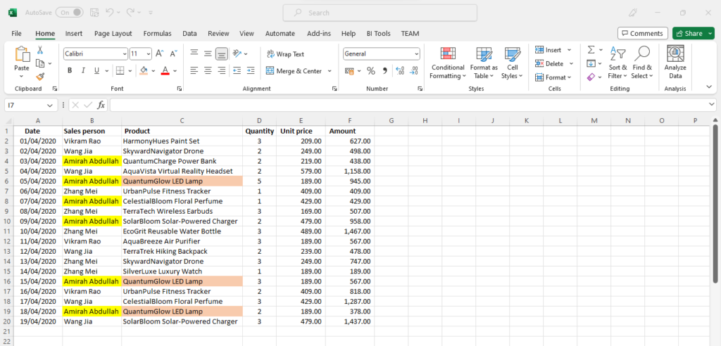
From this, we want to total up sales for Amirah Abdullah, but only for product QuantumGlow LED Lamp.

As you can see from the worksheet, Amirah has sold other products as well, so we need to filter the total sales for only QuantumGlow LED Lamp.

Start by typing in =SUMIFS( in an empty cell.

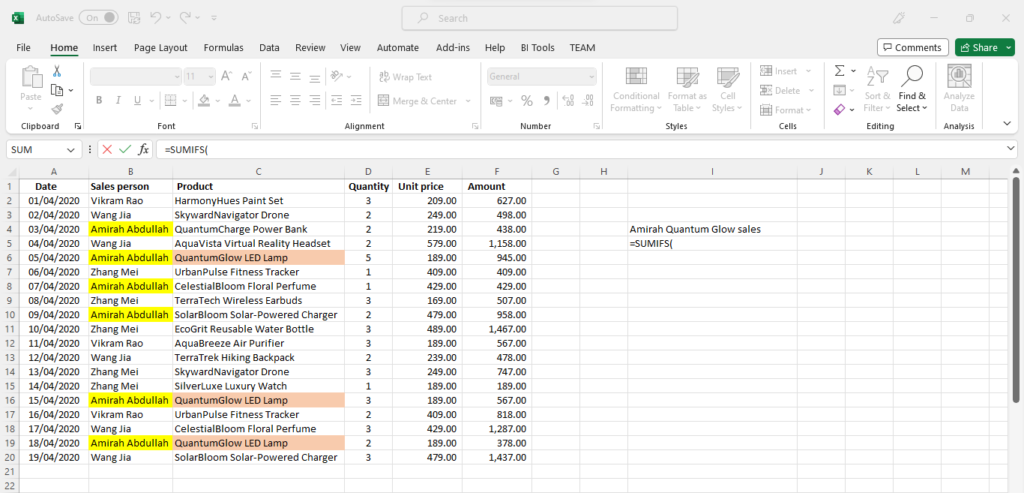
The first thing we need to do is specify the range where the values are that we want to total.

This will be the sum_range in the formula.

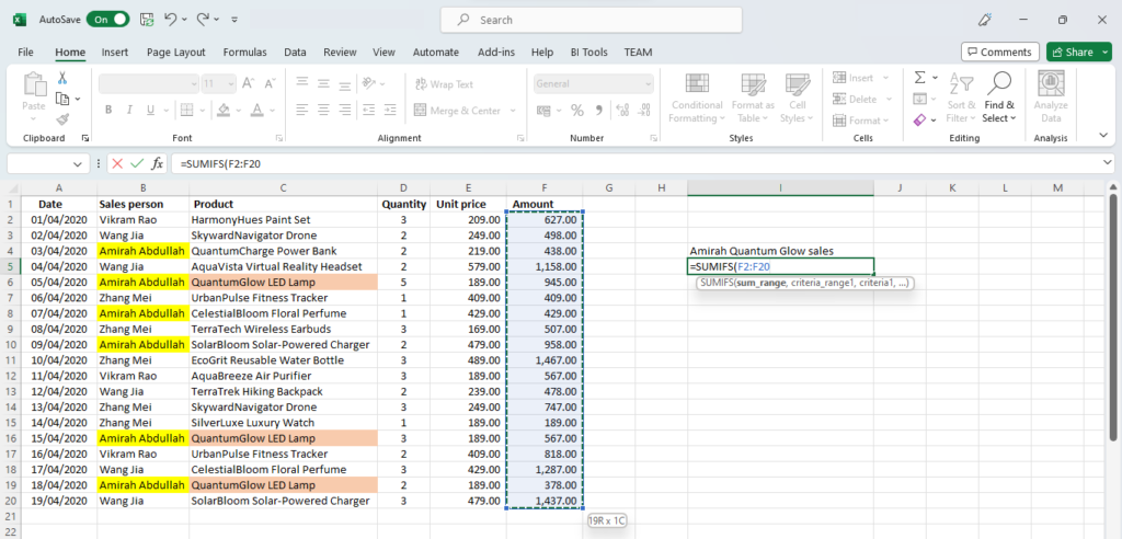
In this case the total sales values are in column F, so we select F2 to F20 and type in a comma to move to the next part in the formula.

Next, we need to select the column where we want to search for the first criteria.

This will be the criteria_range1 part of the formula.

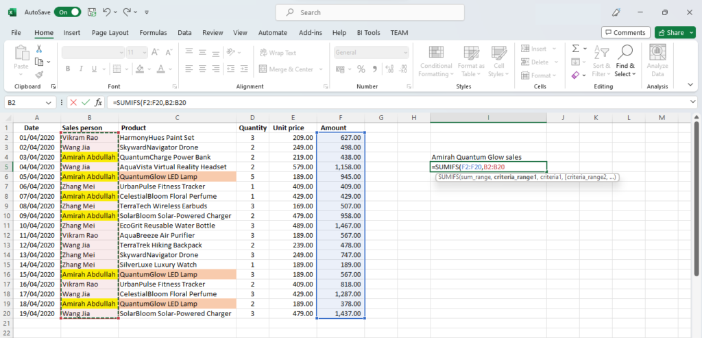
For criteria_range1, we want to look for Amirah Abdullah, and the names of all sales persons are listed in column B.

Select cell B2 to B20 and enter a comma.

Now we need to enter the value that we are looking for in that range, so type in “Amirah Abdullah” followed by a comma.

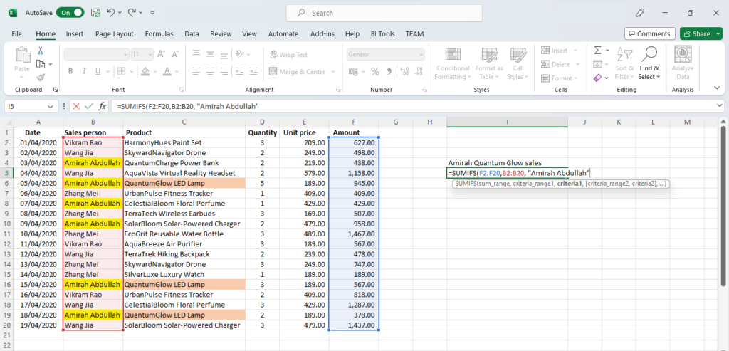
For our second criteria, we want only sales for QuantumGlow LED Lamp.

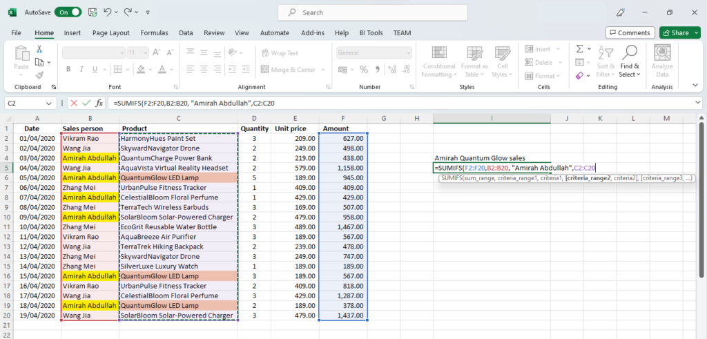
The product names are in column C, so we need to select cells C2 to C20.

Type in a comma, then add the second criteria, “QuantumGlow LED Lamp” and press enter to complete the formula.

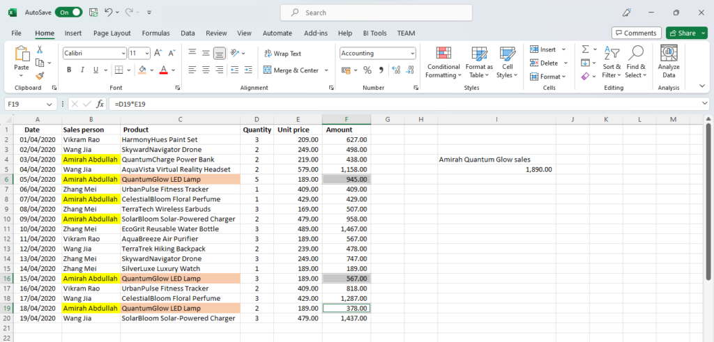
Excel then looks through columns B and C for Amirah Abdullah and QuantumGlow LED Lamp, and if found, adds the sales amount to the total as shown in cell I5.

The completed formula will be:

=SUMIFS(F2:F20,B2:B20,"Amirah Abdullah",C2:C20,"QuantumGlow LED Lamp")

sum_range is F2:F20, the sales amount column which we want to total,

criteria_range1 is B2:B20, the column that has all the sales person’s names,

criteria1 is “Amirah Abdullah”, the sales person we want the total sales for,

criteria_range2 is C2:C20, the column with the product names, and,

criteria2 is “QuantumGlow LED Lamp”, the product sales total that we need for Amirah Abdullah.

Try this out

You can now extend this for other sales persons to find out who made the most QuantumGlow LED Lamp sales.

Also try using wild cards for criteria1 and criteria2.

So instead of keying in the sales persons full name, “Amirah Abdullah”, key in “Amirah*” instead and for criteria2, use “QuantumGlow*“.

This article is also available in: Bahasa Malaysia Bahasa Indonesia