This post is also available in: Bahasa Malaysia (Malay) Bahasa Indonesia (Indonesian)
SUMIF() is similar to SUM(), but it also provides you the ability to specify a condition or criteria so that you can get a total of values that meet the condition.
SUMIF(range, criteria, sum_range)range – this is the range of cells that will contain the criteria you want to check as well as the values you want to sum.
criteria – the condition that you want to check,
sum_range – the range of cells that have the values you want to sum.
For example, if you have a worksheet containing daily sales figures, and wanted a total of sales by state, then you can use the SUMIF() function.
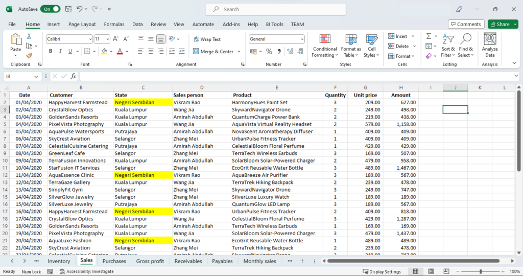
Here, we want a total of sales in Negeri Sembilan.
Select an empty cell where you want to show the total, then type in =SUMIF(.
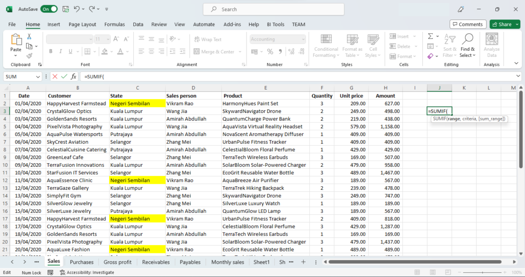
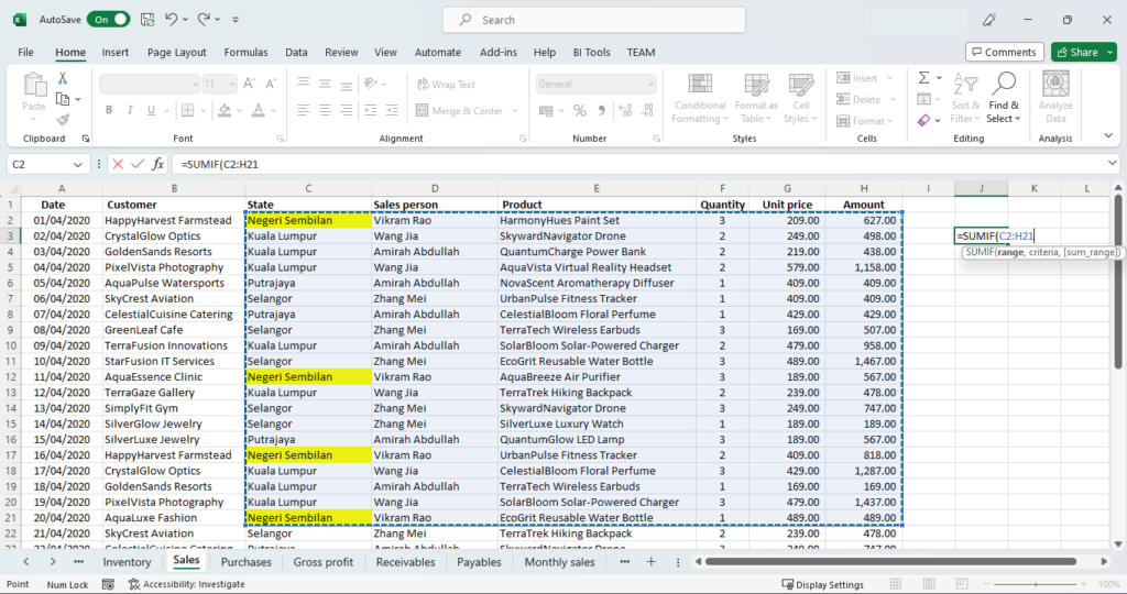
The state name is in column C, while the sales amount is in column H, so for range, select cells C2 to H21.
Next type in a comma, then type in “Negeri Sembilan”.
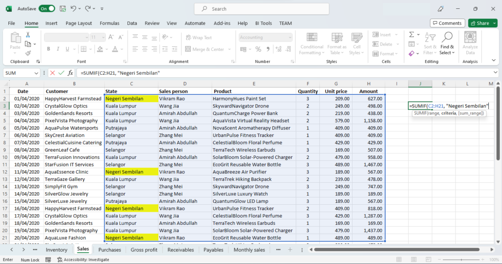
This would be the criteria, or condition that you provide for which you want the total.
Type in another comma, then select the range with the values you want to total.
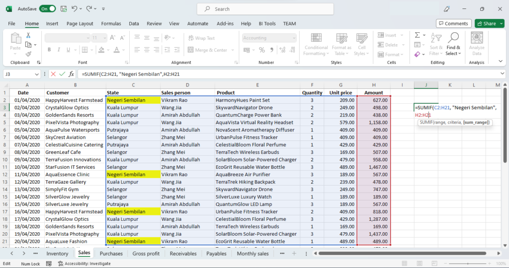
This would be the sum_range, which is the Amount column from H2 to H21.
Your formula will now look like this:
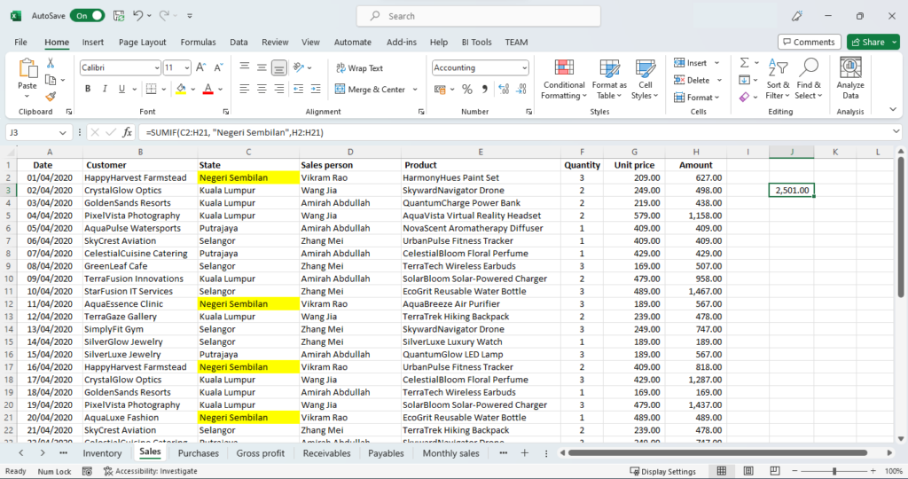
=SUMIF(C2:H21, "Negeri Sembilan",H2:H21)Press enter to complete the formula.
The total of daily sales for Negeri Sembilan will be shown in the cell.
Using wild cards with SUMIF()
If you want to match a broader range with your search criteria, then you can use wild cards.
For example, in the criteria part, if you want a total of sales for all states with names that start with K, you could use “K*”.
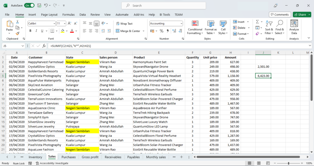
Your formula would look like this
=SUMIF(C2:H21, "K*",H2:H21)This would match and sum for all states with names that start with “K”, and will sum up the sales for Kuala Lumpur, Kedah as well as Kelantan.
